Google Sheets Format Numbers
Number Formats
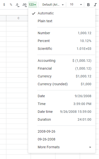
The default Number format is Automatic.
Why change number formats?
- Make data explainable
- Prepare data for functions, so that Google Sheets understands what kind of data you are working with.
Examples of number formats:
- Automatic
- Number
- Currency
- Time
Number formats can be changed by clicking the Number format dropdown (![]() ), accessed in the Ribbon, found in the Numbers group.
), accessed in the Ribbon, found in the Numbers group.

Example
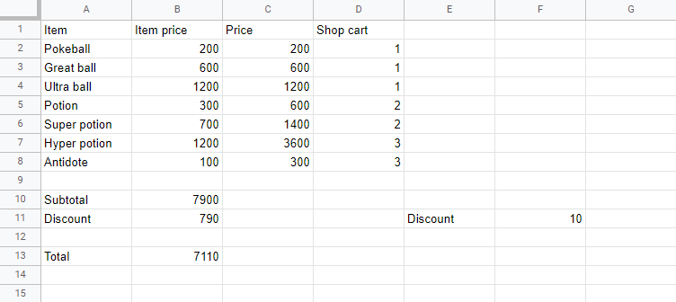
In the example we have cells that represent prices, which can be formatted as Currency.
Copy the values to follow along.
Let's try to change the format of the prices to the Currency Number format.
Step by step:
- Select the range
B2:C8
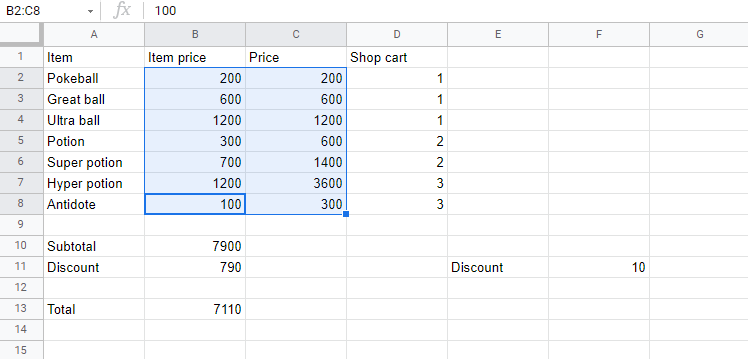
- Click the Number format dropdown menu (
 )
)
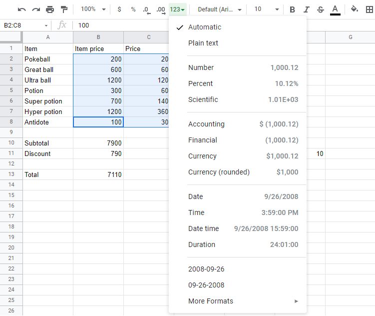
- Click the Currency format

That's it! The Number format was changed from Automatic to Currency.
Note: Google Sheets uses the local currency defined in the location setting.
Now, do the same for cells B10, B11 and B13:
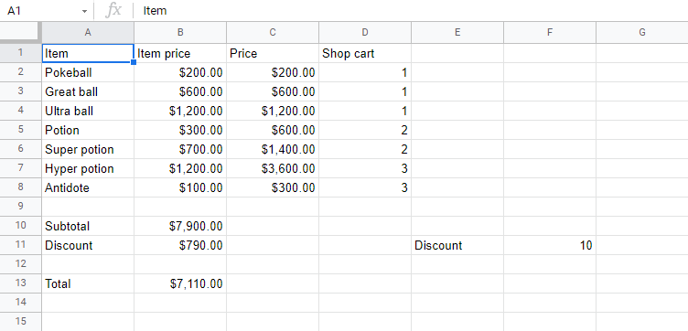
Did you make it?
Note: The currency can be changed. For example instead of using $ like in the example you can decide for NOK or EUR. It is changed in the dropdrop menu, clicking the More Formats in the bottom of the menu. Then, clicking on More Currencies.
Notice that the numbers look like a mess. Let's solve that by decreasing the decimals. This helps to make the presentation more neat.
Decimals
The number of decimals can be increased and decreased.
There are two commands:
- Increase Decimal (
 )
) - Decrease Decimal (
 )
)
Clicking them reduces or increases the number of decimals.
The commands can be found next to the Number format dropdown menu.

Note: Decreasing Decimals can make Google Sheets round up or down numbers as more decimals get removed. This may be confusing if you are working on advanced calculations which require accurate numbers.
Let's clean this up, step by step:
- Select the range
B2:C8 - Click the Decrease Decimal button two times (
 )
)
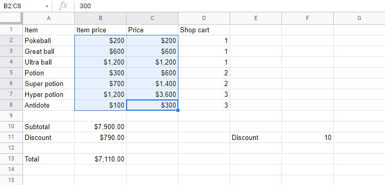
Great!
Do the same for cells B10, B11 and B13:
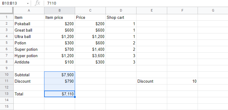
That looks a lot better!
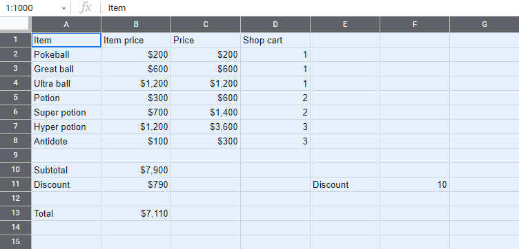
Pro tip: The rectangle in the top left corner by row 1 and column A can be clicked to select all cells in the sheet. This can be useful if you want to change the Number format or change Decimals for all cells.
Chapter summary
Number formats can be changed to make the spreadsheet more understandable or to prepare cells for functions. You can increase and decrease decimals to make the presentation neat.
