Menu
×
   ❮   
HTML CSS JAVASCRIPT SQL PYTHON JAVA PHP HOW TO W3.CSS C C++ C# BOOTSTRAP REACT MYSQL JQUERY EXCEL XML DJANGO NUMPY PANDAS NODEJS R TYPESCRIPT ANGULAR GIT POSTGRESQL MONGODB ASP AI GO KOTLIN SASS VUE DSA GEN AI SCIPY AWS CYBERSECURITY DATA SCIENCE
     ❯   

Excel Tutorial

Excel HOME Excel Introduction Excel Get Started Excel Overview Excel Syntax Excel Ranges Excel Fill Excel Move Cells Excel Add Cells Excel Delete Cells Excel Undo Redo Excel Formulas Excel Relative Reference Excel Absolute Reference Excel Arithmetic Operators Excel Parentheses Excel Functions

Excel Formatting

Excel Formatting Excel Format Painter Excel Format Colors Excel Format Fonts Excel Format Borders Excel Format Numbers Excel Format Grids Excel Format Settings

Excel Data Analysis

Excel Sort Excel Filter Excel Tables Excel Conditional Format Excel Highlight Cell Rules Excel Top Bottom Rules Excel Data Bars Excel Color Scales Excel Icon Sets Excel Manage Rules (CF) Excel Charts

Table Pivot

Table Pivot Intro

Excel Case

Case: Poke Mart Case: Poke Mart, Styling

Excel Functions

AND AVERAGE AVERAGEIF AVERAGEIFS CONCAT COUNT COUNTA COUNTBLANK COUNTIF COUNTIFS IF IFS LEFT LOWER MAX MEDIAN MIN MODE NPV OR RAND RIGHT STDEV.P STDEV.S SUM SUMIF SUMIFS TRIM VLOOKUP XOR

Excel How To

Convert Time to Seconds Difference Between Times NPV (Net Present Value) Remove Duplicates

Excel Examples

Excel Exercises Excel Syllabus Excel Study Plan Excel Certificate

Excel References

Excel Keyboard Shortcuts


Excel Conditional Formatting


Conditional Formatting

Conditional formatting is used to change the appearance of cells in a range based on your specified conditions.

The conditions are rules based on specified numerical values or matching text.

Changing the appearance of cells can visually highlight interesting data points for analysis.

The browser version of Excel provides a number of built-in conditions and appearances:
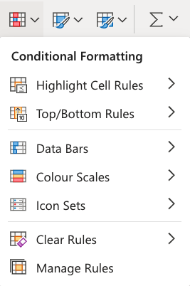
Note: The web browser version of Excel only offers a selection of built-in conditional formatting options.

The Excel application has the option of creating fully customized conditional formatting rules.


Conditional Formatting Example

Here, the Speed values of each pokemon is formatted with a Color Scale:
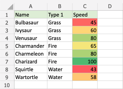
Note: Excel has several different color scales to pick from.


Color Scale Formatting Example

Highlight the Speed values of each Pokemon with Color scale conditional formatting.

Copy Values

Conditional formatting, step by step:

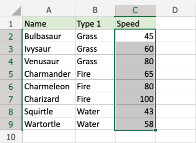
  1. Select the range of Speed values C2:C9
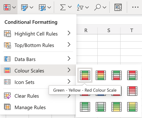
  1. Click on the Conditional Formatting icon in the ribbon, from the Home menu
  2. Select Color Scales from the drop-down menu
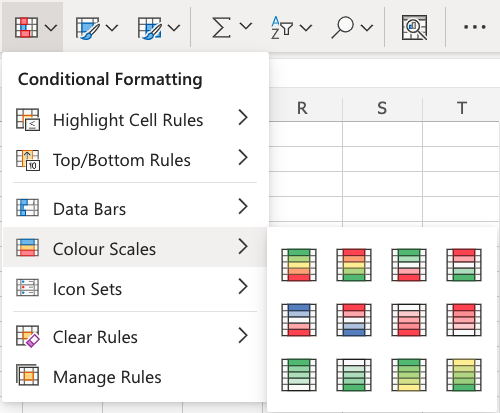
There are 12 Color Scale options with different color variations.

The color on the top of the icon will apply to the highest values.

  1. Click on the "Green - Yellow - Red Colour Scale" icon
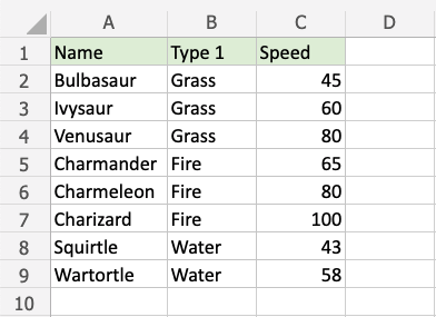
Now, the Speed value cells will have a colored background highlighting:

Dark green is used for the highest values, and dark red for the lowest values.

Charizard has the highest Speed value (100) and Squirtle has the lowest Speed value (43).

All the cells in the range gradually change color from green, yellow, orange, then red.


×

Contact Sales

If you want to use W3Schools services as an educational institution, team or enterprise, send us an e-mail:
[email protected]

Report Error

If you want to report an error, or if you want to make a suggestion, send us an e-mail:
[email protected]

W3Schools is optimized for learning and training. Examples might be simplified to improve reading and learning. Tutorials, references, and examples are constantly reviewed to avoid errors, but we cannot warrant full correctness of all content. While using W3Schools, you agree to have read and accepted our terms of use, cookie and privacy policy.

Copyright 1999-2025 by Refsnes Data. All Rights Reserved. W3Schools is Powered by W3.CSS.